Benchmarking Embedding Models for Semantic Search.

I’m working on a restaurant similarity search engine and leveraging semantic search to deliver more accurate results. The goal is to enable natural language queries — like “cozy brunch spots” or “authentic Mexican food” — and return relevant matches from my dataset. I won’t dive too deep into the mechanics of semantic search in this post, the focus here is on benchmarking different embedding models to find the best fit for my use case. Along the way, I’ll also explain why I decided to replace the original model I was using.

An embedding model is a machine learning model that transforms text into numerical representations (vectors or embeddings), capturing the semantic meaning of words or phrases to enable similarity comparisons. These models have been trained specifically for this sort of task. For instance, a vector could look like this [0.1, 0.2, 0.3, 0.4, 0.5].

The goal of this post is to identify the top-performing embedding model for retrieving restaurants that best match a given search query. By generating vectors for both search queries and restaurant descriptions, we can measure their cosine similarity to evaluate how likely a restaurant is to appear in the search results. Additionally, we’ll fine-tune cosine similarity thresholds to strike the perfect balance between quality (precision) and quantity (recall), ensuring that the results are both accurate and comprehensive.

Understanding metrics

Before diving deeper, let’s take a moment to clarify the metrics we’ll use to evaluate our models. These metrics — precision, recall, and a derived metric called F-score — are key to understanding performance.

If you’re already familiar with these concepts, feel free to skip ahead. For the rest of us, let’s break it down with a simple analogy:

Imagine you’re searching for Italian restaurants, and the algorithm gives you 10 results.

Precision measures accuracy. How many of the 10 results are actually Italian restaurants? If 8 out of 10 are correct, your precision is 80%.
Recall measures coverage. Out of all the Italian restaurants in the database, how many did the algorithm find? If there are 9 Italian restaurants total and the search returns 8 of them, your recall is about 89% (8 out of 9).

Together, these metrics help us assess the balance between quality (precision) and completeness (recall).

But you mentioned a third metric…F-score?

Sometimes, we want a single metric to summarize both precision and recall, especially when we need to balance the two. This is where the F-score comes in. It combines precision and recall into one number by calculating their harmonic mean.

For example, if your precision is 80% and recall is 89%, the F1-score would be approximately 84%. (How to calculate F1)

F1 = 2*(0.8*0.89)/(0.8+0.89) // 0.84

Note: The F1-score assumes that precision and recall are equally important. However, in some cases, you might prioritize one over the other, for example:

If precision is more critical (e.g, reducing false positives in a medical diagnosis system), you may want to place more weight on precision.
If recall is more important (e.g, ensuring no relevant results are missed in a search engine), you may want to prioritize recall instead.

To adjust this balance, you can use the F-beta score, a generalization of the F1-score. (F-beta formula) Where:

beta < 1: Places more emphasis on precision.
beta > 1: Places more emphasis on recall.
beta = 1: Balances precision and recall equally (this is the F1-score).

Let’s get started.

Note: this post was originally a jupyter notebook. You can head over here should you want to run the code directly.

Setting up the notebook

We’re going to import everything that we need for this experiment.

from llama_cpp import Llama
import pandas as pd
import numpy as np
from sklearn.metrics.pairwise import cosine_similarity
from sklearn.metrics import precision_score, recall_score, fbeta_score
import contextlib
import io
import sys
import matplotlib.pyplot as plt

Load up restaurant data

To get started, I’ve provided some sample data from my dataset, conveniently saved as a CSV file. All we need to do is load it up and get to work.

For readers following on this blog post and not on the jupyter notebook, you can download the data here.

pd.set_option('display.max_colwidth', 400)
places_df = pd.read_csv('places.csv')

places_df.head()

id	description	name
1885	Authentic Mexican tacos, prepared by Mexican chefs, now available on Crescent Street and St-Denis Street in Montreal.	Tacos Victor Crescent
6250	La Prep offers a wide variety of fresh, made-to-order meals daily. From pastries to salads and sandwiches, …	La Prep
6797	9th-floor Montreal restaurant with a seaside-themed terrace offering stunning downtown views and H3-signature cuisine & cocktails.	Terrasse Alizé
1937	Unfussy Italian cafe & coffee shop with WiFi, sports on TV & a menu of pizza & pastas until late.	Expresso Bar
6306	Vintage design bar & restaurant with salads, sandwiches, burgers & amuse bouches on the menu.	LOCAL75 Bistro Pub

Most of these restaurant descriptions were either sourced from Google or generated using Gemini, leveraging the metadata I had for each restaurant.

Writing test cases

To effectively evaluate our system, we need to design search queries and identify which restaurants should be retrieved for each query. These queries mimic real-world searches to ensure they align closely with the restaurants in our dataset. By doing this, we can simulate user interactions and assess the system’s performance accurately.

In addition to defining test cases, we’ll also specify the models we want to compare. For this experiment, I’ve selected a variety of all-MiniLM models at different quantization levels and a model from Nomic AI. This will allow us to assess performance across a range of architectures and precision.

test_cases = [
    {
        "query": "Looking for a place with authentic Mexican food.",
        "expected_restaurants": [1885, 7164]
    },
    {
        "query": "Find restaurants with rotisserie chicken",
        "expected_restaurants": [3536, 2439, 3322]
    },
50 collapsed lines
    {
        "query": "Find casual spots with burgers and fries.",
        "expected_restaurants": [
            3191,
            170,
            5330,
            2439,
            1386
        ]
    },
    {
        "query": "Looking for sushi places offering poke bowls.",
        "expected_restaurants": [
            4972,
            6397,
            1097,
            7302,
            1789
        ]
    },
    {
        "query": "Find upscale places with cocktails and unique dishes.",
        "expected_restaurants": [
            6797,
            7462,
            3523,
            6102,
            7164,
            3036,
            7230,
            4593
        ]
    },
    {
        "query": "Where can I find a great brunch spot?",
        "expected_restaurants": [3289, 3966, 5568]
    },
    {
        "query": "Places with sandwiches",
        "expected_restaurants": [
            6250,
            6306,
            1919,
            170,
            6065,
            2231,
            4749,
            5467,
        ]
    }
]

models = [
    {
        "name": "All-MiniLM-L6-v2 Q4_K_S",
        "repo_id": "second-state/All-MiniLM-L6-v2-Embedding-GGUF",
        "filename": "*Q4_K_S.gguf"
    },
    {
        "name": "All-MiniLM-L6-v2 Q4_K_M",
        "repo_id": "second-state/All-MiniLM-L6-v2-Embedding-GGUF",
        "filename": "*Q4_K_M.gguf"
    },
    {
        "name": "All-MiniLM-L6-v2 Q5_K_M",
        "repo_id": "second-state/All-MiniLM-L6-v2-Embedding-GGUF",
        "filename": "*Q5_K_M.gguf"
    },
    {
        "name": "All-MiniLM-L12-v2 Q4_K_M",
        "repo_id": "sheldonrobinson/all-MiniLM-L12-v2-Q4_K_M-GGUF",
        "filename": "*q4_k_m.gguf"
    },
    {
        "name": "nomic-embed-text Q5_K_M",
        "repo_id": "nomic-ai/nomic-embed-text-v1.5-GGUF",
        "filename": "*Q5_K_M.gguf",

        # These are specific to this model
        "query_prefix": "search_query: ",
        "document_prefix": "search_document: "
    },
]

Now, let’s build a set of helper functions to handle the heavy lifting for our experiment. I’ll include clear documentation for each function to help you understand its purpose and functionality.

def load_model(repo_id, filename, **kwargs):
    """
    Simple wrapper around `from_pretrained`. llama-cpp will take care of downloading the model using huggingface-hub.
    You can manage the models locally using their CLI.
    """
8 collapsed lines
    return Llama.from_pretrained(
            repo_id=repo_id,
            filename=filename,
            verbose=False,
            embedding=True,
            n_gpu_layers=1,
            **kwargs
        )

def load_model_without_warning(repo_id, filename, **kwargs):
    """
    Wrapper around `load_model` which silences some warnings about unsupported kernels.
    We can safely ignore these warnings as it really pertains to the hardware this notebook is running on.
    """
16 collapsed lines
    buffer = io.StringIO()
    with contextlib.redirect_stderr(buffer):
        llm = load_model(repo_id, filename, **kwargs)

    captured_output = buffer.getvalue().splitlines()

    # llama-cpp writes directly to stderr/stdout but it keeps printing warning about messages that can be ignored such as
    # ggml_metal_init: skipping kernel_get_rows_bf16                     (not supported)
    for line in captured_output:
        if "ggml_metal_init: skipping kernel_" in line:
            continue
        else:
            # Print back anything that's not the kernel warning
            print(line, file=sys.stderr)

    return llm

def normalize_vectors(vectors):
    """
    Normalize vectors using the Euclidean norm.
    Each vector will have a magnitude of 1.
    This makes sure cosine similarity doesn't get skewed towards vectors with a big magnitude as we only care about vector direction.
    """
2 collapsed lines
    norms = np.linalg.norm(vectors, axis=1, keepdims=True)
    return vectors / norms


def generate_embeddings(llm, docs, prefix=""):
    """
    Generate embeddings using llama-cpp and the current loaded model.
    Note: some embedding models require to add a task prefix in front of the document to embed. e.g `search_document: {doc}`
    """
3 collapsed lines
    docs = [f"{prefix}{doc}" for doc in docs]
    response = llm.create_embedding(docs)
    return normalize_vectors([k['embedding'] for k in response['data']])


def generate_model_results(
    llm,
    places,
    test_cases,
    document_prefix = "",
    query_prefix = "",
):
    """
    Generate a dataframe with various metadata about each place, as well as a cosine similarity score given the current query and each restaurant.
    We will generate various metrics from this dataframe.
    """
28 collapsed lines
    # Shape (50,384)
    embeddings = generate_embeddings(llm, places['description'].tolist(), document_prefix)

    results = []
    for case in test_cases:
        query = case["query"]
        expected_restaurants = case["expected_restaurants"]

        # Shape (1,384)
        query_embedding = generate_embeddings(llm, [query], query_prefix)

        # Shape (1,50)
        cosine_similarities = cosine_similarity(query_embedding, embeddings)[0]

        # Shape (1,50)
        # Normalizing a [-1,1] range into [0,1] score whereas 1 is completely identical.
        cosine_scores = (cosine_similarities + 1) / 2

        for idx, score in enumerate(cosine_scores):
            results.append({
                "query": query,
                "expected_in_search": places.iloc[idx]['id'] in expected_restaurants,
                "description": places.iloc[idx]['description'],
                "restaurant_id": places.iloc[idx]['id'],
                "score": score
            })

    return pd.DataFrame(results)

def analyze_thresholds(test_cases, results_df, f_beta=1, thresholds=np.linspace(0, 1, 50)):
    """
    Evaluates precision, recall, and F-beta for each search query at various cosine similarity thresholds.
    Returns an analysis that includes the most optimal threshold, which maximizes the F-beta score based on the chosen weighting.

    Note: You can specify a custom F-beta value to adjust the balance between precision and recall:
  •  F-beta < 1: Emphasizes precision.
  •  F-beta > 1: Emphasizes recall.
    """
43 collapsed lines
    threshold_analysis = {}

    # Group results by query
    grouped_results = results_df.groupby('query')

    for query, group in grouped_results:
        # Find corresponding test case
        test_case = next(tc for tc in test_cases if tc['query'] == query)

        fbeta_scores = []
        precisions = []
        recalls = []

        # Test each threshold
        for threshold in thresholds:
            y_true = group['expected_in_search']

            # Note: This can yield only `False` value if the threshold is too high, e.g 1.00
            # As a result, sklearn can complain if it doesn't see some labels in `y_pred` when calculating metrics.
            y_pred = group['score'] >= threshold

            precision = precision_score(y_true, y_pred, zero_division=np.nan)
            recall = recall_score(y_true, y_pred)
            fbeta = fbeta_score(y_true, y_pred, beta=f_beta)

            fbeta_scores.append(fbeta)
            precisions.append(precision)
            recalls.append(recall)

        # Find optimal threshold
        best_idx = np.argmax(fbeta_scores)
        optimal_threshold = thresholds[best_idx]

        threshold_analysis[query] = {
            'optimal_threshold': optimal_threshold,
            'fbeta': {
                'value': fbeta_scores[best_idx],
                'precision_at_value': precisions[best_idx],
                'recall_at_value': recalls[best_idx]
            }
        }

    return threshold_analysis

Measuring Performance

Now it’s time to evaluate each query against all the models and measure their performance. For this, we’ll:

Load each model: Loop through all selected models, initialize them and generate embeddings.
Create the necessary dataframes: Prepare the data for analysis, including cosine similarity scores for each query and restaurant pairing.
Perform threshold analysis: Identify the optimal cosine similarity thresholds yielding the best f-beta score.
Prepare reporting data: Generate a consolidated dataset that summarizes the results, ready for reporting and comparison.

This should give you a good overview at the performance of each model for individual queries.

rows = []

for model_info in models:
    llm = load_model_without_warning(repo_id=model_info["repo_id"], filename=model_info["filename"])
    query_prefix = model_info.get("query_prefix", "")
    document_prefix = model_info.get("document_prefix", "")
    results_df = generate_model_results(llm, places_df, test_cases, document_prefix, query_prefix)
    threshold_analysis = analyze_thresholds(test_cases, results_df, f_beta=1)

    for query, analysis in threshold_analysis.items():
        rows.append({
            "model_name": model_info["name"],
            "query": query,
            "best_threshold": analysis["optimal_threshold"],
            "best_fbeta": analysis["fbeta"]["value"],
            "recall_from_fbeta": analysis["fbeta"]["recall_at_value"],
            "precision_from_fbeta": analysis["fbeta"]["precision_at_value"],
        })

df = pd.DataFrame(rows)
df.head()

Pairing each models to each queries and measuring individual performance. Remember, each query is tested against all of the restaurant descriptions, which is what ultimately is represented below. The dataframe should look something like this:

model_name	query	best_threshold	best_fbeta	recall_from_fbeta	precision_from_fbeta
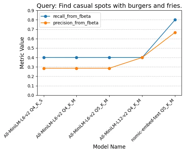
All-MiniLM-L6-v2 Q4_K_S	Find casual spots with burgers and fries.	0.714286	0.333333	0.400000	0.285714
All-MiniLM-L6-v2 Q4_K_S	Find restaurants with rotisserie chicken	0.775510	0.500000	0.333333	1.000000
All-MiniLM-L6-v2 Q4_K_S	Find upscale places with cocktails and unique dishes.	0.734694	0.500000	0.500000	0.500000
All-MiniLM-L6-v2 Q4_K_S	Looking for a place with authentic Mexican food.	0.755102	1.000000	1.000000	1.000000
All-MiniLM-L6-v2 Q4_K_S	Looking for sushi places offering poke bowls.	0.755102	1.000000	1.000000	1.000000

Analysis

While we could simply pick the model with the highest average F1-score and call it a day, it would be interesting to take a look deeper. By analyzing how each individual model performs on specific queries, we can uncover their strengths and weaknesses.

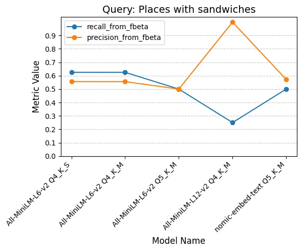
We can plot the performance of each model on each of the individual queries.

queries = df['query'].unique()
metrics = ['recall_from_fbeta', 'precision_from_fbeta']

for query in queries:
    query_data = df[df['query'] == query]

    plt.figure(figsize=(6, 5))

    for metric in metrics:
        plt.plot(
            query_data['model_name'],
            query_data[metric],
            marker='o',
            label=metric
        )

    plt.title(f"Query: {query}", fontsize=14)
    plt.yticks(np.arange(0, 1, 0.1))
    plt.xlabel("Model Name", fontsize=12)
    plt.ylabel("Metric Value", fontsize=12)
    plt.grid(axis='y', linestyle='--', alpha=0.7)
    plt.xticks(rotation=45, ha="right")
    plt.legend()
    plt.tight_layout()
    plt.show()

I won’t show all individual queries here, you can view them in the jupyter notebook.

Examining the performance of each model per query reveals some interesting patterns. While All-MiniLM-L6-v2 Q4_K_S, All-MiniLM-L6-v2 Q4_K_M, and All-MiniLM-L6-v2 Q5_K_M show similar results, All-MiniLM-L12-v2 Q4_K_M appears to lean more towards optimizing for precision at the expense of recall. On the other hand, nomic-embed-text Q5_K_M seems to prioritize recall slightly more than precision.

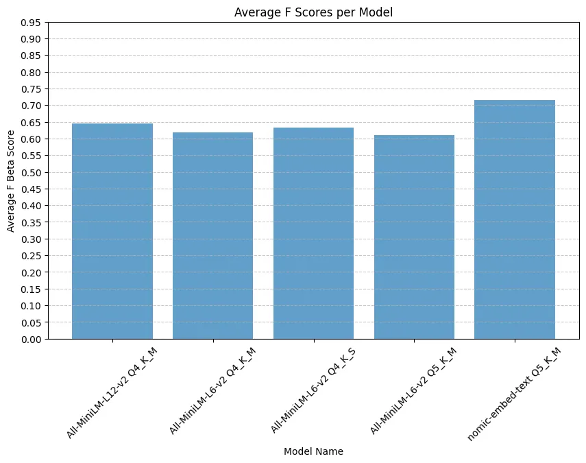
We can now take the mean F-beta score for each model. This will give us a clearer picture of which model performs better overall, balancing precision and recall according to our chosen F-beta weighting.

avg_metrics = df.groupby("model_name").agg(
    avg_fbeta=("best_fbeta", "mean")
).reset_index()

model_name	avg_fbeta
All-MiniLM-L12-v2 Q4_K_M	0.644589
All-MiniLM-L6-v2 Q4_K_M	0.617367
All-MiniLM-L6-v2 Q4_K_S	0.631653
All-MiniLM-L6-v2 Q5_K_M	0.609524
nomic-embed-text Q5_K_M	0.715801

plt.figure(figsize=(10, 6))
plt.bar(avg_metrics["model_name"], avg_metrics["avg_fbeta"], alpha=0.7)
plt.title("Average F Scores per Model")
plt.xlabel("Model Name")
plt.ylabel("Average F Beta Score")
plt.xticks(rotation=45)
plt.yticks(np.arange(0, 1, 0.05))
plt.grid(axis='y', linestyle='--', alpha=0.7)
plt.show()

Performance plot of the average F Scores per Model

The nomic-embed-text model stands out with the best F-beta score, showcasing a balanced approach between precision and recall. However, our earlier per-query analysis suggests that if we shifted from a balanced F1 to a weighted F-beta (F < 1) emphasizing precision, All-MiniLM-L12-v2 Q4_K_M might emerge as the top performer. This highlights how the choice of model ultimately depends on what’s most valuable in your specific context—precision, recall, or balance.

It’s also worth noting that nomic-embed-text benefits from a larger context window, which we’re not fully leveraging. Utilizing longer descriptions could further enhance this model’s accuracy and overall performance.

Conclusion

The goal of this experiment was to compare various embedding models to identify the best performer for our restaurant similarity search. We evaluated restaurant descriptions against a variety of search queries using cosine similarity, determining the most appropriate thresholds for each model and query.

By analyzing the overall performance of each model through their respective F-beta scores, we found that the nomic-embed-text model from Nomic AI outperformed the others when using an equally weighted F1 score. Its balanced approach to precision and recall, combined with its larger context window, makes it particularly well-suited for this task, especially if longer descriptions are utilized.

This analysis highlights not only the overall best-performing model but also the trade-offs between precision and recall across different models. It emphasizes the importance of tailoring the choice of model to the specific needs of the application—whether that means prioritizing precision, recall, or maintaining a balance between the two.

I hope you enjoyed reading this analysis. As always, you can send me any questions or feedback, I’d be happy to answer!